3  RStudio Software

How to use quantitative data analysis software

Abstract

This chapter introduces researchers to R and RStudio, the primary tools used throughout this playbook for data analysis and reporting. Researchers learn the distinction between R (the underlying programming language) and RStudio (the interface used to write and run R code), then walk through downloading and installing both programs on Mac or Windows. The chapter covers RStudio’s four main panels — the console, script editor, environment, and files/plots/packages/help tab — and explains how each is used in a typical workflow. Researchers also learn the difference between working in the console versus writing reusable code in a script, how to use an RStudio Project so that the working directory is set automatically for importing and saving files, and how to create and organize a Quarto document (.qmd) using code chunks and comments. The chapter closes with a list of common beginner errors and their fixes, preparing researchers to troubleshoot independently as they begin working with real data in later chapters.

Keywords

start, RStudio, install R, console, script, RStudio project, working directory

ResourcesResources: RStudio

• Posit RStudio
• R4DS RStudio
• Cheatsheet page
• Cheatsheet PDF
• Fávero, L. P., Belfiore, P., & De Freitas Souza, R. (2023). Introduction to R-based language. In Data Science, Analytics and Machine Learning with R (pp. 7–25). Elsevier. https://doi.org/10.1016/B978-0-12-824271-1.00033-0

GoGo: You have already run R code

In Coding a Plot, you ran R code in your web browser. In this chapter you put R on your own computer, so that you can run code with your own data, save your work, and write your reports.

3.1 What is R and RStudio?

R is a programming language used for statistical computing and quantitative data analysis. RStudio is a user-friendly interface that makes it easier to write and run R code. R performs the computations, data manipulation, and calculations, while RStudio provides tools that help you organize and execute your code. You will need both R and RStudio on your computer to do quantitative data analysis. Once you download both R and RStudio programs, you will NOT need to open and use R. You will use RStudio to do all of your computational programming.

Things you can do in RStudio:

• Run commands
• Perform statistical analysis tests
• Make plots
• Publish reports
• Clean and manipulate data
• Create interactive websites

3.2 Downloading R and RStudio

Because RStudio runs on top of R, R must be installed before installing and using RStudio.

3.2.1 Download R

R comes from a website called CRAN (the Comprehensive R Archive Network). It is a plain, text-only page, and that is normal.

1. Go to https://cran.r-project.org/.

2. At the top of the page, under Download and Install R, click the link for your computer: “Download R for macOS” or “Download R for Windows”.

   

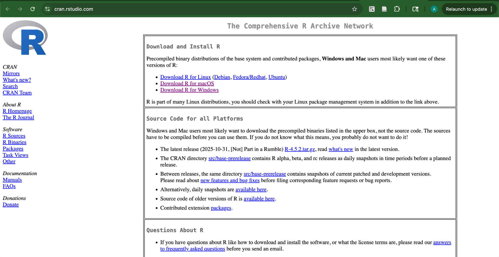
   The CRAN home page

3. Follow the instructions below for your computer. The version number you see (for example, R-4.6.1) will be higher than in these screenshots, because R is updated a few times a year. That is fine: always take the newest version.

Mac

1. Click “Download R for macOS.”

2. Under Latest release, there are two packages. Download the one that matches your chip: For Apple silicon (M1, M2, …) Macs or For older Intel Macs.

   GoHint: Apple silicon or Intel?

   To see if your Mac is silicon or Intel, go to the Apple icon on the top left corner and select About This Mac. If you see Chip followed by Apple M1, M2, M3, or M4, it is silicon; if it says Processor followed by Intel Core, it is Intel.

   

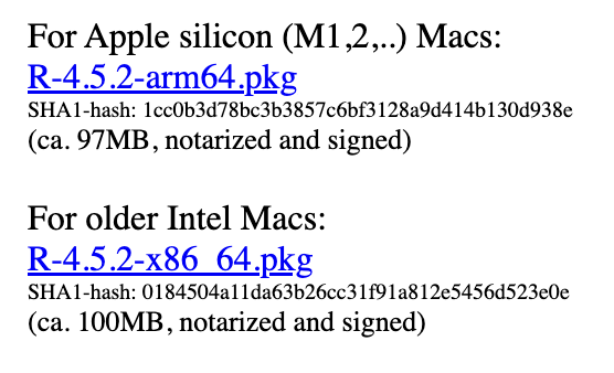
   Choose the package that matches your Mac (your version number will be newer)

3. Open the downloaded .pkg file and click Continue through the installer, the same way you install other apps. If your Mac asks whether the installer may access your Downloads folder, click Allow.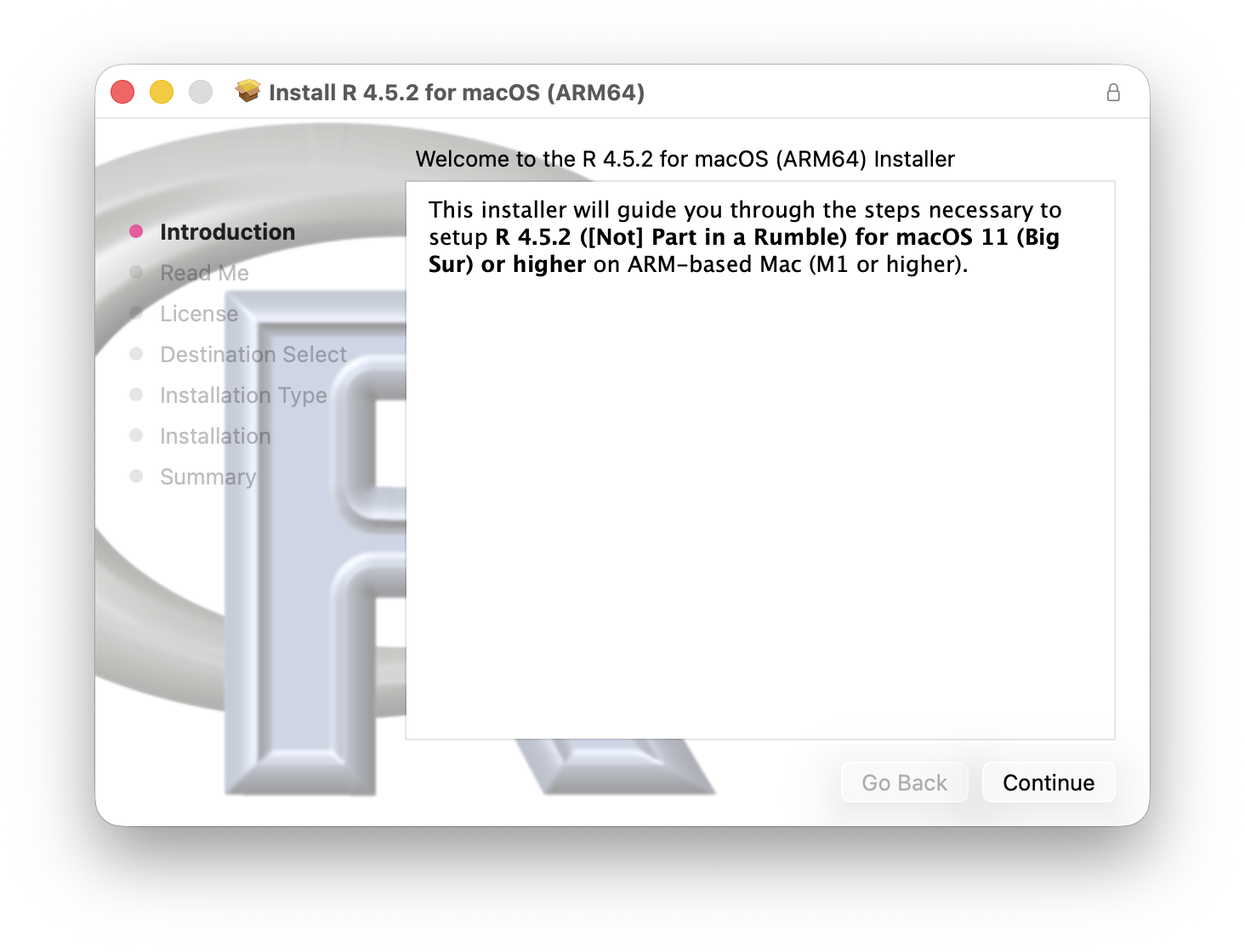

   

   The R installer for macOS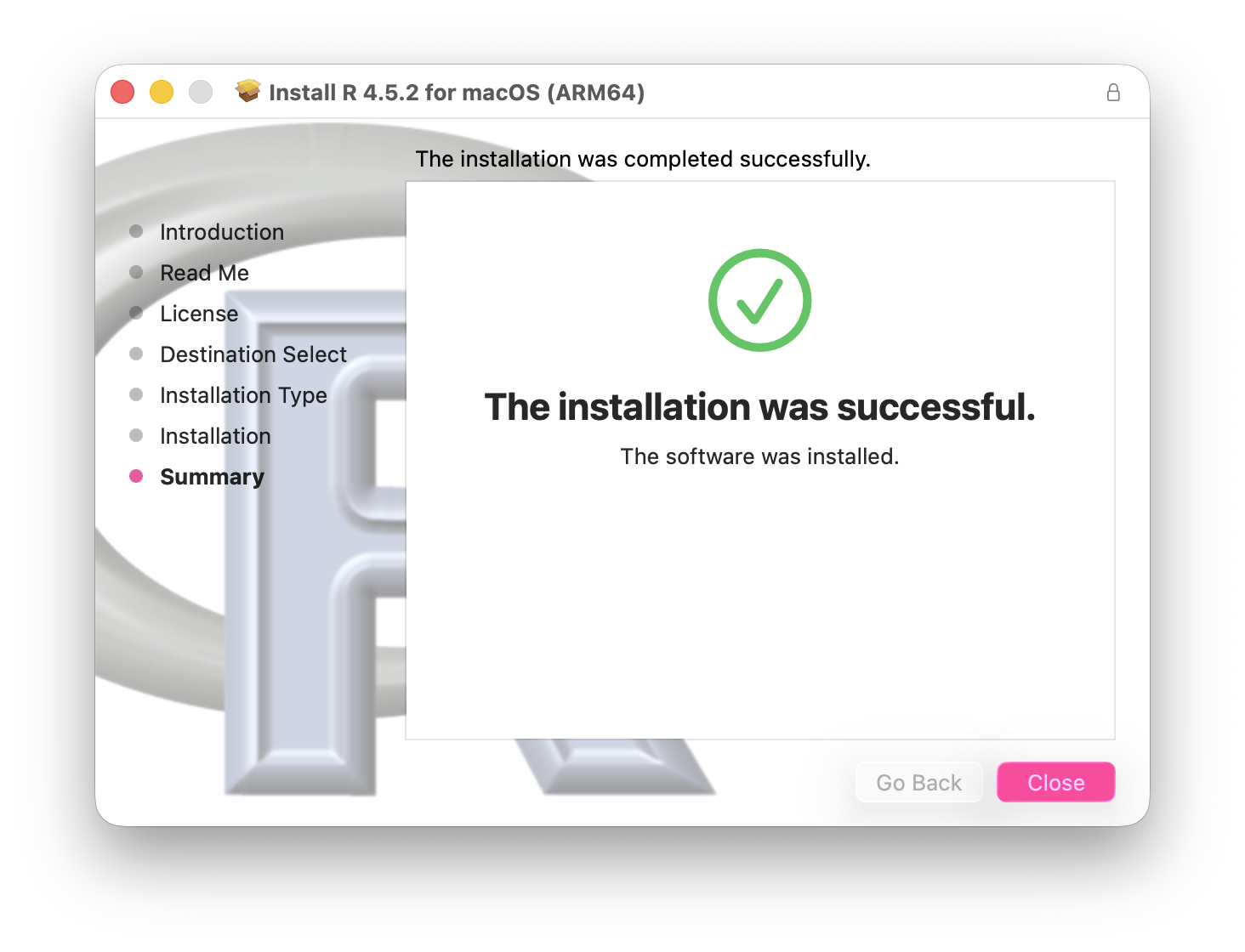

   

   The installation was successful

Windows

1. Click “Download R for Windows.”

2. Click “install R for the first time.”

   

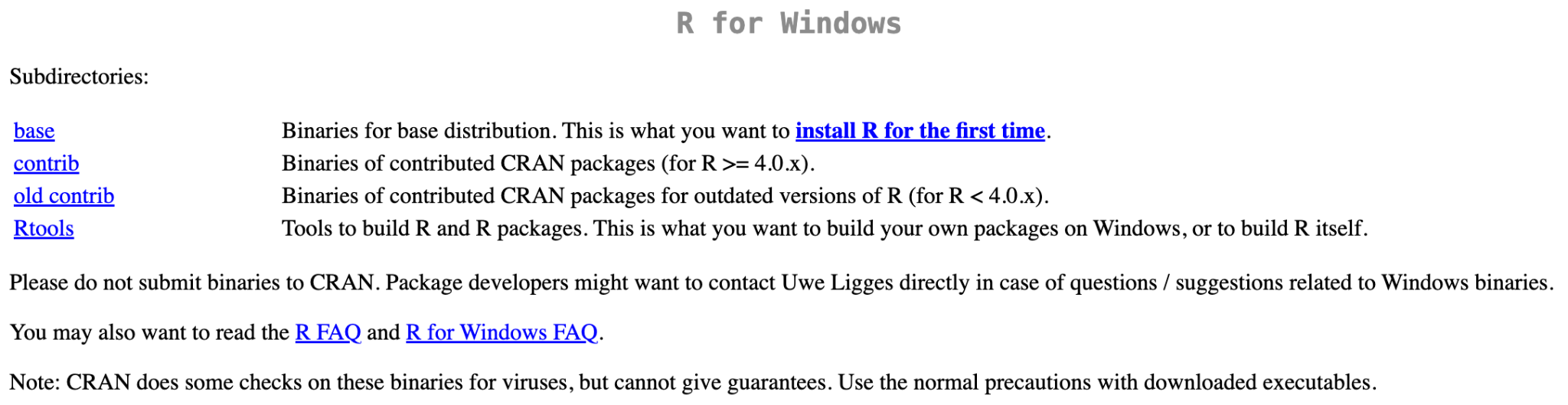
   The R for Windows page on CRAN

3. Click the large link at the top of the page, “Download R-4.x.x for Windows” (the version number changes over time).

4. Open the downloaded .exe file and click Next through the installer. The default settings are fine.

3.2.2 Download RStudio

1. Go to https://posit.co/download/rstudio-desktop/. This address now opens the RStudio IDE User Guide on Posit’s documentation site. Do not be surprised: that is the right page.

2. Scroll down to the heading Direct Downloads (Open Source). You will see a table with one row per operating system.

3. Click the file in the Download column that matches your computer:

   • Mac: the row macOS 14+, a .dmg file.
   • Windows: the row Windows 11, an .exe file (not the zip archive).

   The file name includes a version number such as 2026.09.0. Newer is fine.

4. Open the downloaded file and follow the prompts, the same way you install other apps. On a Mac, drag the RStudio icon into the Applications folder when the window asks you to.

5. Open RStudio. It should look like this:

   

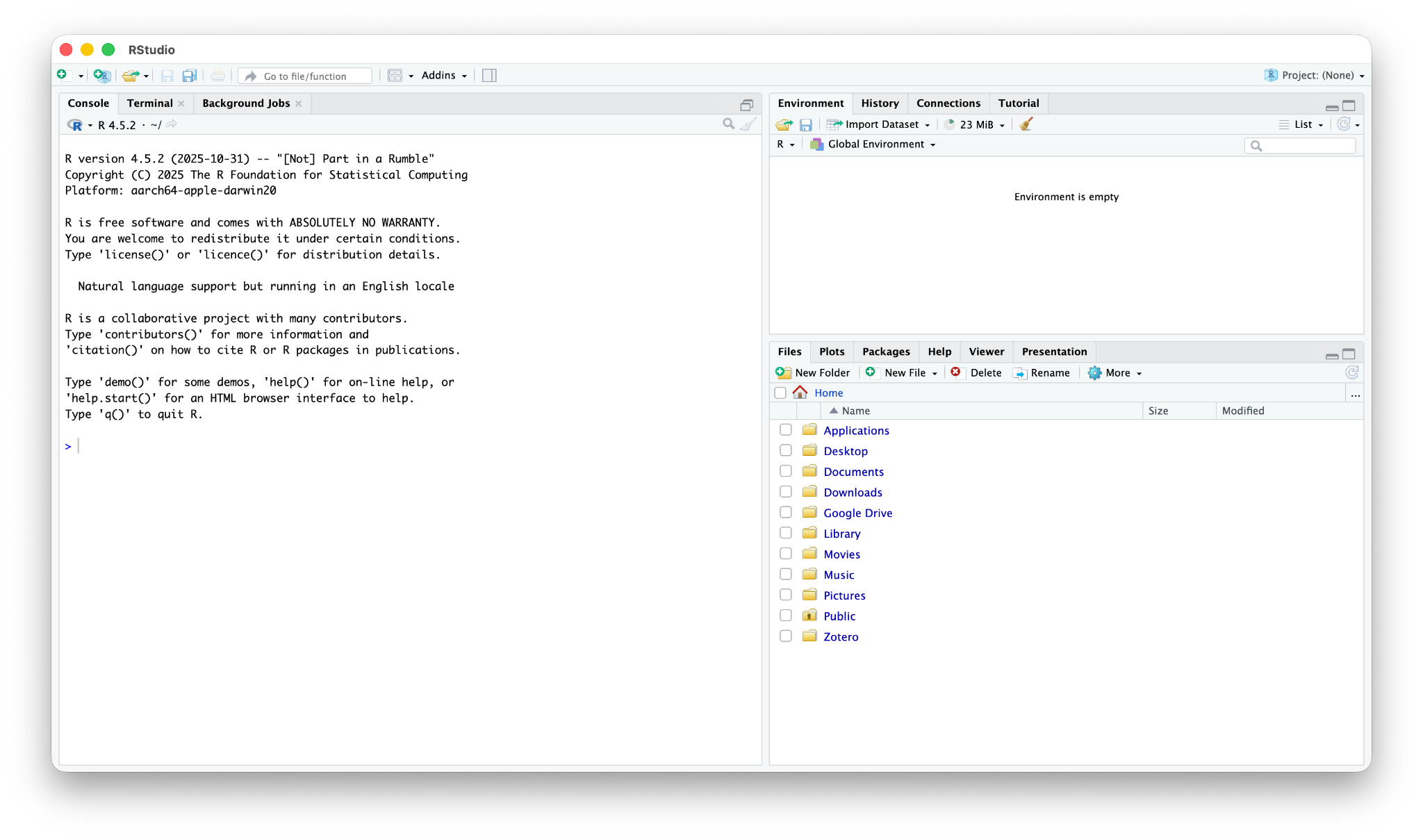
   RStudio when you open it for the first time

CautionCaution: Older computers

The download table lists macOS 14+ and Windows 11. If your computer is older than that, ask a peer mentor and/or Dr. Shane before class: there are older RStudio versions that still work, and the FRI lab computers have RStudio installed.

3.3 Navigating the Layout

When you open RStudio, the default window looks like the image below. You will see four main panels.

Figure 3.1: The four main panels of RStudio

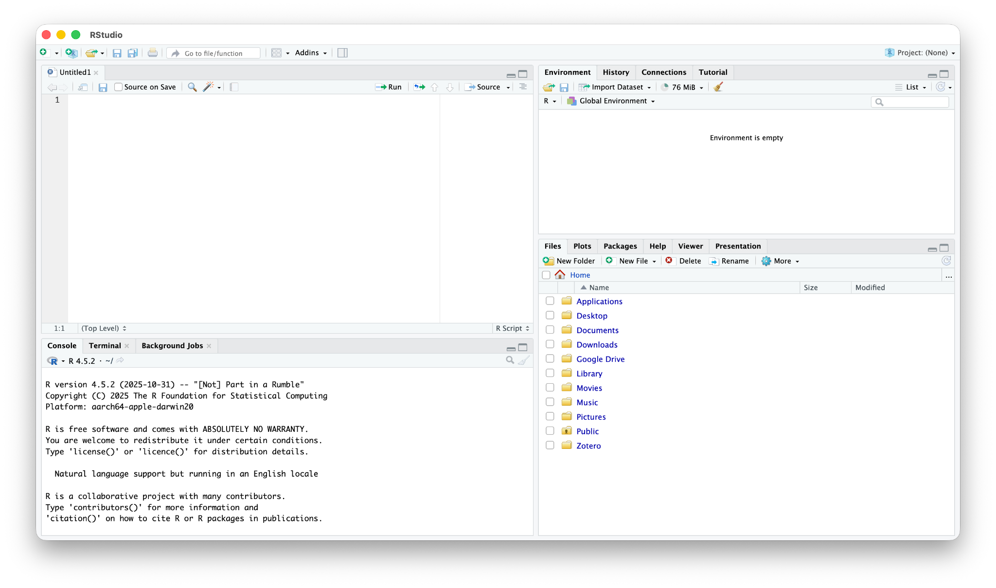
The lower left corner has three important tabs. The main section here is the console. Commands can be typed directly into this section and R will execute them immediately. All code executed during each R session will be displayed in this section, along with any outputs. Any errors that may happen will also appear here. It is important to note that any work in the console does not get saved. In order to save code, it must be written in the script editor. The terminal is another tab located in this section. In this class, the terminal is used to publish our reports as Quarto websites. The background jobs tab shows longer tasks that RStudio runs in the background, such as rendering or previewing a Quarto document.

The script editor is in the upper left corner. A script is a file that contains code. Commands can be typed into the script to be saved and returned to later. When commands are run in the script editor, their outputs will appear in the console.

The upper right corner is the environment tab. Any objects created and saved in R will appear here. For example, we will see any imported or created data sets and variables. This panel also contains the history tab, which keeps a list of the commands you have run.

There are many tabs located in the lower right corner. The files tab allows us to navigate files and folders in the entire directory. This is where we will import any new files and data. The plots tab will display any graphs or images generated by code in the current session. The packages tab lists all the installed R packages. The help tab provides R documents and tutorials for functions and packages.

3.4 Scripts and Quarto Documents

3.4.1 Three places to write code

You can type R code in three places in RStudio, and each one has a job.

Where	What happens to the code	Use it for
Console (bottom left)	Runs immediately. Not saved. Gone when you close RStudio.	Quick checks and one-time commands: getwd(), head(alldata), looking up a value, installing a package.
.R script	Saved as a file. Runs when you click Run or Source. Code only, with # comments.	Code that is not part of any report, such as your install.R file.
.qmd Quarto document	Saved as a file. Runs when you click Render. Code chunks and your writing in one file, which becomes a web page.	Everything for your RD Report and Final Report: every import, plot, and analysis.

Think of the console as scratch paper and the two file types as the notebook. Scratch paper is the right place to try one line or check a number. Nobody keeps scratch paper.

ImportantImportant: Write your analysis in a .qmd file, not in the console

In this course, all of the code for your reports goes in code chunks inside your .qmd file. Here is why.

• It can be checked. Your peer mentor, Dr. Shane, your teammates, and later readers can open your .qmd and see exactly how every number and plot was made. Code typed in the console leaves no record, so nobody can review it, and neither can you.
• It can be published. Rendering a .qmd turns your code, results, and writing into one web page with a URL, which is what you submit (Publish). A console session cannot be published.
• It can be redone. Render runs every chunk from a fresh start, so your report proves that the analysis works from top to bottom. That is what reproducible means, and it is the point of Reproducible Reports.
• It keeps the explanation next to the code. A .qmd holds your Methods and Results paragraphs beside the code that produced them, so the writing and the numbers cannot drift apart.

Use the console to try things. When a line works and belongs in your analysis, put it in a chunk in your .qmd.

3.4.2 Scripts

A script is a text file that contains code. It allows us to enter commands and save our work, then return to it later. Unlike the console, where commands run immediately and are not saved, scripts allow us to store a set of commands for future use or sharing. In this course the one script you need is install.R (R Packages).

3.4.3 Creating and saving a new script

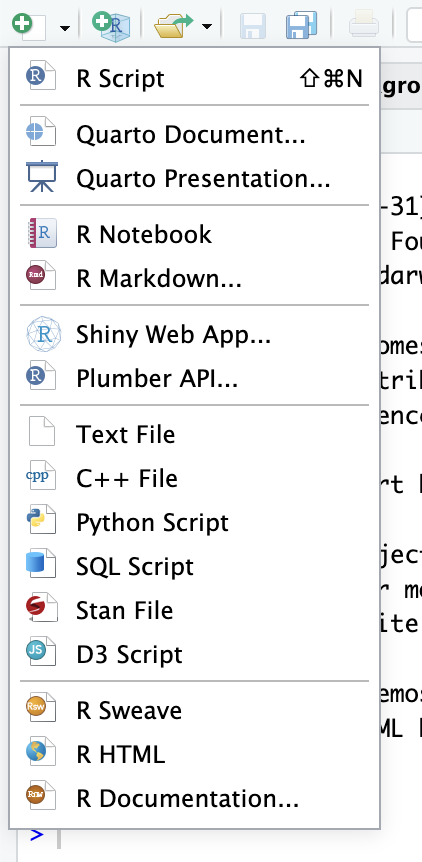
In the upper left hand corner, press the green icon with the plus sign, then click “R Script.” A blank script will appear in the script editor.

To save a new script, press the single disk icon in the toolbar. A pop-up should appear to save the script. Name the file and save it to the appropriate place.

The New File menu

3.4.4 RStudio Projects and the Working Directory

The working directory is the folder on your computer where R looks for files and saves new ones. If the file you want to import is not in the working directory, R will not be able to find it and you will see a “cannot open file” error.

The easiest way to manage the working directory is to let RStudio do it for you with an RStudio Project. A project is simply a folder on your computer that contains a small .Rproj file. Whenever you open the project, RStudio automatically sets the working directory to that folder. You will keep everything for your individual report — data files, R scripts, and Quarto documents — together in this one folder.

The rest of this section has three parts: what you set up once, what you do every time you work, and two important guidelines about where your files go.

Set up once: create your project

1. Click File > New Project…
2. Choose New Directory, then New Project.
3. For Directory name, type Lastname_FRI (using your own last name, with no spaces).
4. For Create project as subdirectory of, click Browse and choose a place you can find again, such as your Documents folder.
5. Click Create Project. RStudio restarts inside your new project.

You will know you are in your project when its name (Lastname_FRI) appears in the top right corner of RStudio, and the files tab shows the contents of your project folder, including the file Lastname_FRI.Rproj.

Every time: open your project and start clean

Always start your work by opening the project, not an individual file. You can either:

• double-click the Lastname_FRI.Rproj file in your project folder (Finder on Mac or File Explorer on Windows), or
• in RStudio, click File > Open Project… (or use the project menu in the top right corner) and select your .Rproj file.

To confirm that the working directory is your project folder, copy and paste this code into the console (which is the tab in the bottom left corner of RStudio) and then press “return” (on a mac) and “enter” on a windows computer:

getwd()

GoGo: Start each session with a clean slate

Change this setting once, and it protects every session after that. Go to Tools > Global Options > General. Under Workspace, uncheck “Restore .RData into workspace at startup” and set “Save workspace to .RData on exit” to Never. This way, your results always come from the code in your script or Quarto document rather than from leftover objects.

How folders are nested, on your computer and in RStudio

A folder can hold files and other folders, and those folders can hold more. Your computer shows this as a path: the list of folders you open, one inside the next, to reach a file. On a Mac the path to a data file might be /Users/shane/Documents/McCarty_FRI/data/10.09.2026.team1.cleandata.xlsx; on Windows, C:\Users\shane\Documents\McCarty_FRI\data\10.09.2026.team1.cleandata.xlsx. Read it from left to right: the Users folder holds shane, which holds Documents, which holds McCarty_FRI, which holds data, which holds the file.

An RStudio Project turns that long path into a short one. When the project is open, RStudio stands inside McCarty_FRI, so every path you type starts there. "data/10.09.2026.team1.cleandata.xlsx" means “the data folder inside the project, and the file inside it”. That is why every import line in this playbook starts with data/ and no line ever starts with /Users/ or C:\. The same project folder works on any computer, including your peer mentor’s and your instructor’s, because the path is relative to the project, not to the computer.

This is the whole layout of a project for this course. Nothing else goes in the root (the project folder itself), and nothing goes anywhere but the two subfolders:

McCarty_FRI/                          <- the project folder: open it by double-clicking the .Rproj
├── McCarty_FRI.Rproj                 <- the project file RStudio made
├── install.R                         <- run once per computer (R Packages)
├── lab_prep.R                        <- the lab cleaning script, next to the .Rproj, NOT in data/
├── McCarty_lab2.qmd                  <- one .qmd per lab (Start a Report)
├── McCarty_lab3.qmd
├── McCarty_lab4.qmd
├── McCarty_lab5.qmd
├── McCarty_RDreport.qmd              <- the report (Start My Report)
├── McCarty_finalreport.qmd           <- a copy of the RD report, later
├── readme.qmd                        <- for publishing (Read Me)
├── references.bib                    <- Zotero export (Citations & Refs)
├── apa.csl                           <- APA style file (Citations & Refs)
├── data/                             <- EVERY data file: the lab files and your team's .cleandata file
│   ├── ANTH306_LayConceptionsMH_SYNTHETIC.xlsx
│   └── 10.09.2026.team1.cleandata.xlsx
└── plots/                            <- EVERY plot you save with ggsave() (Write the Results)
    ├── plot1_wellbeing_treated_barplot.png
    └── plot2_stigma_helpseek_scatter.png

RStudio’s Files tab (bottom right) shows this same tree, one level at a time: click a folder to go into it, and click the project name in the path at the top of the tab to come back out. Rendering a .qmd adds an .html file next to it; that is expected and you do not need to move it.

Important guidelines: where your files go

Every data file you use must be inside your project folder, in a subfolder named data. A file that is still in your Downloads folder, on your Desktop, or in Google Drive is not in your project, and R will not find it. “Move the file into your project folder” means exactly that. Your project folder is an ordinary folder on your computer (the one you created in Finder or File Explorer, which contains Lastname_FRI.Rproj). You move files into it the way you move any file on your computer: in Finder or File Explorer, not inside RStudio. RStudio’s Files tab is only a window that shows what is in that folder, so once the file is there, it appears in the tab on its own.

GoGo: How to move a data file into your project folder

1. Download the file. Get the data file from Brightspace or your team’s Google Drive. Your computer saves it in the Downloads folder.

2. Make the data folder, if you have not yet. In RStudio’s Files tab (bottom right), click New Folder, name it data (lowercase), and click OK. Every data file lives in this folder, and every import line in the playbook starts with "data/…" because of it. You make it once.

3. Open your project folder. In RStudio’s Files tab (bottom right), click the gear icon labeled More and choose Show Folder in New Window. Your project folder opens in Finder (Mac) or File Explorer (Windows).

4. Drag the file in. Open your Downloads folder in a second window, open the data folder inside the project folder window, and drag the data file into data (not next to Lastname_FRI.Rproj; that is where your .qmd and .R files go). (Dragging moves the file. If you would rather keep a copy in Downloads, hold Option on a Mac or Ctrl on Windows while you drag.)

5. Check. Go back to RStudio. Click data in the Files tab and the file appears inside it. If it does not, click the refresh icon at the top right of the Files tab.

Save your R scripts and Quarto documents in the same folder (File > Save As will already point there when the project is open).

Because the working directory is the project folder, you can import data using just the file name:

alldata <- read_excel("data/10.09.2026.team1.cleandata.xlsx")

ImportantImportant: Save your Quarto documents in the project folder

When a Quarto document (.qmd) is rendered, R looks for data files starting from the folder where the .qmd file is saved. If your .qmd file and your data file are both in your project folder, the file name alone will work in the console and when you render.

CautionCaution: Avoid setwd() and full file paths

You may see code that sets the working directory by hand or imports a file with its full location on one person’s computer:

setwd("/Users/yourname/FRI")
read.csv("/Users/yourname/Downloads/alldata_vaccinations.csv")

This code only works on that one computer. It will fail on your teammates’ computers and on your peer mentor’s or Dr. Shane’s computer, because the folder /Users/yourname/ does not exist there. With a project and file names only, the same code runs for everyone who has the project folder.

3.4.5 Quarto

Quarto is a publishing system that allows us to combine text and code to produce reports, presentations and websites. Quarto documents are made using .qmd files. To open a .qmd file and begin a Quarto document, press the green plus sign in the upper left hand corner, then click “Quarto Document.” Quarto documents are saved the same way as scripts.

A .qmd file has two faces. In RStudio you see plain text with a few markers: a header between --- lines, # for headings, and code chunks between ```{r} and ```. When you click Render, Quarto runs the code and turns the text into a finished report: a web page with a title, headings, formatted paragraphs, citations, and your results filled in. Here are the two faces of the same file, from a report by one of this playbook’s authors:

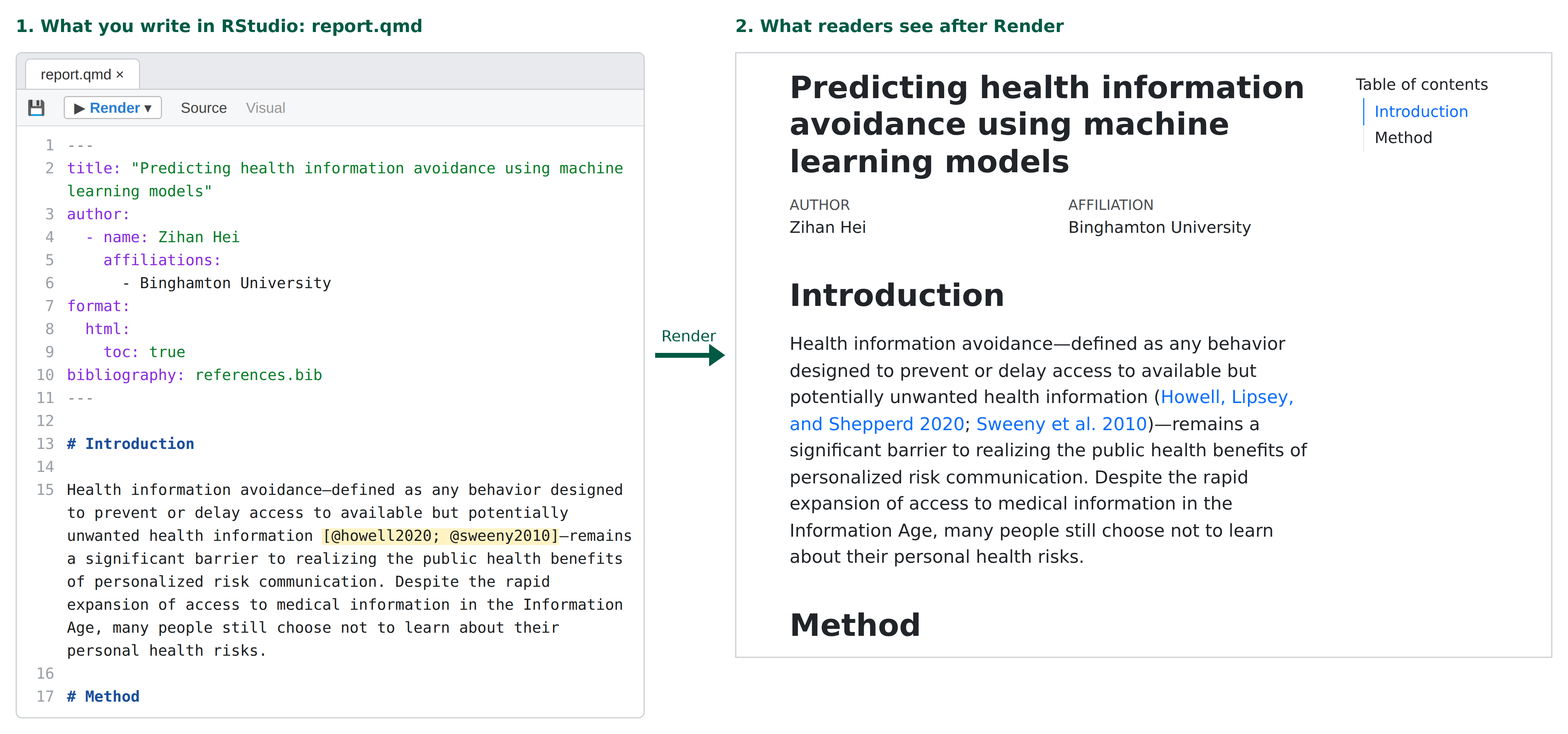
The same report as a .qmd file in RStudio (left) and as the published report (right). Source: Hei, Z. (2025). Predicting health information avoidance using machine learning models. https://zihanhei.quarto.pub/avoider-report/

Notice three things. The YAML header at the top of the file (lines 1 to 11) became the title, author, and table of contents. # Introduction and # Method became headings. And the citation keys [@howell2020; @sweeny2010] (highlighted) became real citations, “Howell, Lipsey, and Shepperd 2020; Sweeny et al. 2010,” which also appear in a reference list at the end. You type plain text; Render does the formatting.

Text written normally in Quarto appears as regular text in the output. In order to include and run code in your RD Report and Final Report, code must be written in code chunks.

The first time you render a Quarto document, RStudio may ask to install packages it needs (such as rmarkdown and knitr). Click Yes.

ResourcesResources: Everything about Quarto reports is in one chapter

This section is only an introduction. Start a Report walks you through the header, code chunks, labels, captions, and comments step by step, and its Resources box links to the Quarto guides you will need.

CautionCaution: Save your file before you close RStudio

RStudio does not save your .qmd or .R file for you. If the file name on its tab is red with a *, your latest changes exist only on the screen, and closing RStudio throws them away. Two different questions come up when you quit, and they need opposite answers.

Do this

• Press Cmd + S (Mac) or Ctrl + S (Windows) every few minutes, and always before you Render. The file name on the tab turns black when it is saved.
• Before you quit, click File > Save All.
• If RStudio asks “Save changes to report.qmd?”, click Save. That question is about your file.
• Copy your .qmd and .R files to your ELN at the end of every session (Find the Ref).

Do not do this

• Do not close RStudio, or your laptop, while a file name is still red.
• Do not click Don’t Save when the question names a file (report.qmd, install.R). Only the question about the workspace (.RData) gets Don’t Save: the workspace is leftovers, and your file is the recipe.
• Do not rely on Render to save for you. It usually does, but only for the file you rendered, and only if the render starts.

3.4.6 Running code

Code in the editor does nothing until you send it to the console. There are three sizes of “run”, and you will use all three.

• One line or a few lines. Put the cursor on a line, or highlight several lines, then click Run or press Cmd + Enter (Mac) / Ctrl + Enter (Windows). This is the everyday way to work: write a line, run it, look at the result.
• One chunk (in a .qmd file). Click the green ▶ arrow in the top right corner of the chunk. The gray ▼ next to it is Run All Chunks Above, which runs every chunk before this one, in order.
• The whole file. For an .R script such as install.R, click Source at the top right of the editor. It runs the file from the first line to the last. For a .qmd report, the whole-file button is Render (see the Quarto section above), which does the same thing and then builds the report.

GoGo: When the whole file stops with an error, run it in pieces

Source and Render stop at the first error. The console shows the error message, but it does not always make clear which line caused it, especially when the message is about a missing package or an object that was never created. When that happens, do not guess and do not rewrite the file. Go back to the top and run it in pieces: one chunk at a time with the green arrow, or a few lines at a time with Cmd/Ctrl + Enter. The first piece that fails is where the problem is, and the lines above it are now known to work. Then use the checklist in Common errors below and the small-mistakes routine from Coding a Plot (Step 5, Find the foul).

3.4.7 Organizing scripts

Lines that start with # are comments: notes to yourself and other readers that R shows but does not run. A comment above each section of a script says what that section is for, which makes a long script easier to read and makes it easier to find the right place when an error message points you back to it. Comments are also how you record the source of your code and explain it in your own words, which are requirements for your reports. Here is the idea in three lines:

# IMPORT: read the team data file
survey <- read.csv("alldata_vaccinations.csv")
head(survey)   # CHECK: the first six rows

You will see comments in practice in the next chapter, R Packages, where the install.R file has one comment for each step of the workflow. Start a Report then explains comments in detail when you build your first code chunk, including the #source: and #explanation: lines your reports need.

3.4.8 Common errors

As you begin working in RStudio, you may encounter some errors. These are normal and can usually be fixed easily. A list of common errors is below:

• Object not found → This means that the object (such as a variable or dataset) has not been created yet. Make sure you have run the code that defines the object before trying to use it.
• Cannot open file → This usually means that RStudio cannot find the file you are trying to import. Check that you have opened your RStudio Project, that the file is in your project folder, and that the file name is spelled exactly right (including the file type, such as .csv).
• Could not find function → This error occurs when a function is not recognized. This is often because a package has not been loaded. Make sure you have run library(thepackagename) before using functions from that package.
• There is no package called… → This means the package has not been installed yet. Run install.packages("thepackagename") to install it, then library(thepackagename) to load it.

3.5 Summary

3.5.1 Terminology

• Console: The area where R runs code and displays output
• Script: A file where code is written and saved for later use
• Object: Any item created and stored in R, such as a variable, dataset, or result of a calculation
• Working Directory: The folder where RStudio looks for and saves files
• RStudio Project: A folder with an .Rproj file; opening it sets the working directory to that folder automatically
• Environment: Displays all objects (such as variables and datasets) created during a session
• Package: A collection of functions and tools that extend R’s capabilities
• Function: A command that performs a specific task
• Quarto Document: A file used to create reports that combine code, output, and text