17  Describe Your Data

How to check whether your outcome is normally distributed

Abstract

This chapter is the first step on the Analysis Map. Researchers check the distribution of the outcome in their research question with a histogram, a Q-Q plot, and the Shapiro-Wilk test, and then decide whether to use a parametric test (normal data) or a non-parametric test (data that are not normal).

Keywords

normality, distribution, histogram, Q-Q plot, Shapiro-Wilk, parametric, non-parametric

Resources Ref’s kickoff: find the Ref before you code

Open Project → Open .qmd → Run load-library chunk → Run All Chunks Above → code. If anything looks wrong, use Ref’s Quick Checklist.

17.1 Why check for normality?

Most statistical tests come in two versions.

• Parametric tests (t-test, ANOVA, Pearson correlation) assume that your outcome is normally distributed. On a histogram, normal data look like a bell: most people are in the middle, and fewer people are at each end.
• Non-parametric tests (Mann-Whitney U, Wilcoxon, Kruskal-Wallis, Spearman correlation) do not make that assumption.

So before you choose a test on the Analysis Map, you need one answer: is my outcome normal, or not?

GoGo: Check the outcome in your research question

You do not need to check every variable in your dataset. Check the outcome: the score your research question is about.

17.2 The example data

This chapter uses the lab dataset and three outcomes:

• WELLBEING: the average of eight items (a composite score from 1 to 5)
• STIGMA_PUB: public stigma, the average of four items (a composite score from 1 to 5)
• HELPSEEK: one item with answers from 1 to 5

library(tidyverse)
source("lab_prep.R")   # creates mh_clean

17.3 Check 1: Look at a histogram

Always start here. Ask: is it roughly bell-shaped, with one hump in the middle?

ggplot(data = mh_clean,
       mapping = aes(x = WELLBEING)) +
  geom_histogram(binwidth = 0.25, fill = "#005a43", color = "white") +
  xlab("Positive mental well-being (1 to 5)") +
  ylab("Number of people") +
  theme_bw()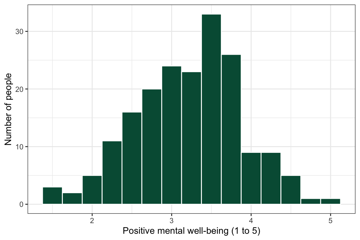

Figure 1. Histogram of the well-being composite score.

ggplot(data = mh_clean,
       mapping = aes(x = STIGMA_PUB)) +
  geom_histogram(binwidth = 0.25, fill = "#005a43", color = "white") +
  xlab("Public stigma (1 to 5)") +
  ylab("Number of people") +
  theme_bw()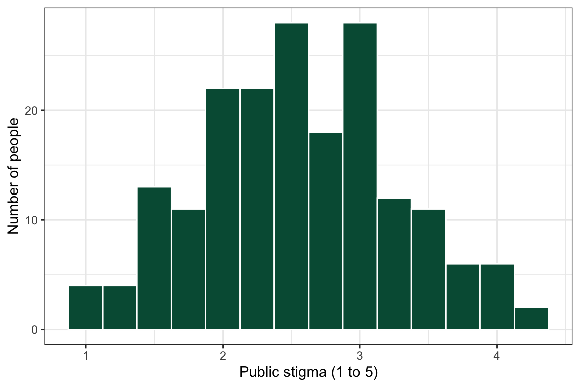

Figure 2. Histogram of the public-stigma composite score.

ggplot(data = mh_clean,
       mapping = aes(x = HELPSEEK)) +
  geom_histogram(bins = 5, fill = "#005a43", color = "white") +
  xlab("Help seeking (1 to 5)") +
  ylab("Number of people") +
  theme_bw()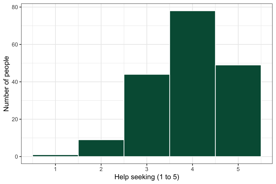

Figure 3. Histogram of the single help-seeking item.

CautionCaution: A single survey item is not normal

One item with only five possible answers cannot make a smooth bell. Treat a single item as not normal and use the non-parametric test. A composite score (the average of several items) has many more possible values and is often close to normal. The more items in the composite, the smoother the histogram.

17.4 Check 2: Look at a Q-Q plot

A Q-Q plot compares your data to a perfect normal distribution. If the points follow the line, the data are close to normal. If the points bend away from the line, especially at the ends, the data are not normal.

ggplot(data = mh_clean,
       mapping = aes(sample = WELLBEING)) +
  geom_qq() +
  geom_qq_line() +
  theme_bw()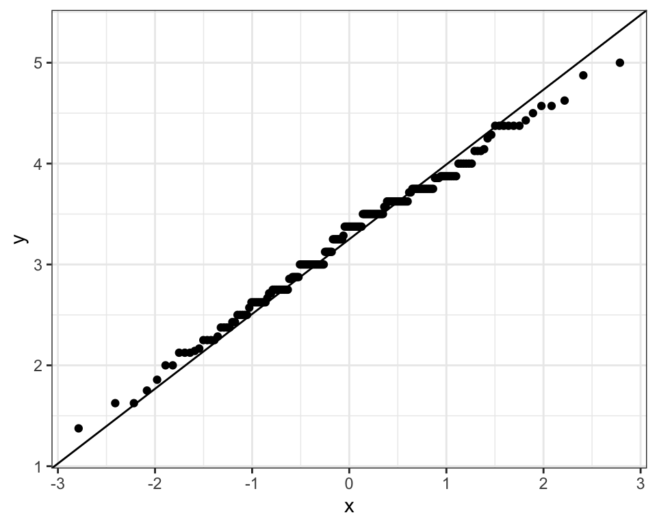

Figure 4. Q-Q plot of the well-being composite score.

ggplot(data = mh_clean,
       mapping = aes(sample = STIGMA_PUB)) +
  geom_qq() +
  geom_qq_line() +
  theme_bw()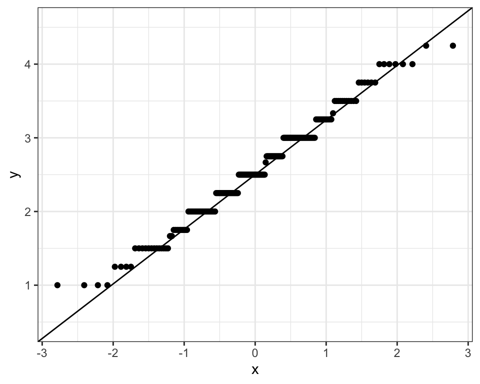

Figure 5. Q-Q plot of the public-stigma composite score.

17.5 Check 3: Run the Shapiro-Wilk test

The Shapiro-Wilk test puts a number on what you saw in the plots.

shapiro.test(mh_clean$WELLBEING)

    Shapiro-Wilk normality test

data:  mh_clean$WELLBEING
W = 0.99136, p-value = 0.3234

shapiro.test(mh_clean$STIGMA_PUB)

    Shapiro-Wilk normality test

data:  mh_clean$STIGMA_PUB
W = 0.98259, p-value = 0.01997

shapiro.test(mh_clean$HELPSEEK)

    Shapiro-Wilk normality test

data:  mh_clean$HELPSEEK
W = 0.86006, p-value = 7.013e-12

How to read the p-value. This one feels backwards, so read it slowly.

• p is larger than .05 → the data are not different from normal → treat the outcome as normal.
• p is smaller than .05 → the data are different from normal → treat the outcome as not normal.

Reading the example. WELLBEING is normal: the histogram is a bell, the Q-Q points follow the line, and the Shapiro-Wilk p-value (0.323) is larger than .05. HELPSEEK is also easy: the histogram is piled up at one end, and p is far below .05. It is not normal. STIGMA_PUB is harder. The histogram has one hump in the middle and no long tail, and the Q-Q points stay close to the line, but the Shapiro-Wilk p-value (0.020) is below .05. Look closely and you can see why: the average of four items on a 1-to-5 scale can take only a few values, so the bar heights jump around instead of rising and falling smoothly, and the Q-Q plot climbs in steps. The checks do not fully agree, so the safe decision is not normal. (The full 8-item STIGMA score, which has twice as many possible values, passes all three checks: more items make a smoother composite.)

CautionCaution: Do not use the Shapiro-Wilk test by itself

With a large sample, the test flags tiny differences that do not matter. With a small sample, it can miss big ones. Use the histogram and the Q-Q plot together with the test. When the three checks disagree, or when you are unsure, choose the non-parametric test and talk to your peer mentor and/or Dr. Shane.

17.6 Make the decision

What you found	Your outcome is	Use the
Bell-shaped histogram, points follow the Q-Q line, Shapiro-Wilk p larger than .05	normal	parametric test (listed under NORMAL on the Analysis Map)
Skewed or lumpy histogram, points bend away from the Q-Q line, Shapiro-Wilk p smaller than .05	not normal	non-parametric test (listed under NOT NORMAL on the Analysis Map)
A single survey item (for example, 1 to 5)	not normal	non-parametric test

Write your answer in your data analysis plan, and report it in your methods:

The distribution of ________ was checked with a histogram, a Q-Q plot, and the Shapiro-Wilk test (W = ___, p = ___). The data were ________ (normal / not normal), so a ________ test was used.

CautionCaution: Don’t pick the test that gives you the result you want

Decide normal or not normal before you run your statistical test, and keep that decision.

ResourcesOne exception: regression

For a linear regression, you check the residuals of the model, not the raw outcome. See Relate 3+ Variables.

Resources Ref’s final whistle: before you quit RStudio

Save → Render → Back up to ELN → Quit, Don’t Save workspace. Details: Ref’s Quick Checklist.